Getting started with `pymultieis`

pymultieis is a Python package for processing multiple electrochemical impedance spectroscopy (EIS) data. It uses an object oriented approach and is based on the torch library. pymultieis provides a Multieis class with methods for fitting, visualizing and saving the results thereafter.

The following steps are good starting points towards analyzing your own data using pymultieis

Hint

Please do not hesistate to open an issue should you encounter any difficulties or notice any bugs.

Step 1: Installation

pymultieis should be installed via PyPI

pip install pymultieis

Step 2: Load your data

The data which is loaded should comprises a vector of frequencies at which the immittance data was taken, and the 2-D array of complex immittances (impedances or admittances) where the size of the rows correspond to the length of the frequencies vector and the size of the columns is the number of spectra to be fitted. If we know the standard deviation of our immittance measurements, this can also be used instead of the modulus or other weighting options. It is assumed that the frequencies are equal for all the spectra in a particular series. The frequencies and immittance shall be our freq and Z when we create our Multieis instance. In the example below the files which were originally stored as numpy arrays will be converted to torch tensors using the torch.as_tensor() function.

We assume that we have our files in the data folder one step above working directory

import numpy as np
import torch
import pymultieis as pym

# Load the frequency data
>>> F = torch.as_tensor(np.load('../data/redox_exp_50/freq_50.npy'))

# Load a 2-D array of admittances to be fitted
>>> Y = torch.as_tensor(np.load('../data/redox_exp_50/Y_50.npy'))

# Load a 2-D array of the standard deviation of the admittances
# Here we assume we know the standard deviation of our admittances.
>>> Yerr = torch.tensor(np.load('../data/redox_exp_50/sigma_Y_50.npy'))

# We can check for the consistency in the shapes of the data we loaded
print(F.shape)
print(Y.shape)
print(Yerr.shape)

torch.Size([45])
torch.Size([45, 50])
torch.Size([45, 50])

Important

pymultieis does not offer a module to parse files. However this can easily be done using Pandas and other available libraries.

Step 3: Define your impedance/admittance model

Next we define our equivalent circuit/immittance model as a normal python function. This approach eliminates the need for prebuilt circuit models and offers researchers a far greater flexibility since any custom immittance function can be fitted to their data.

For instance we shall convert modified Randles circuit shown below to a python function which returns the admittance of the circuit.

A modified Randles circuit

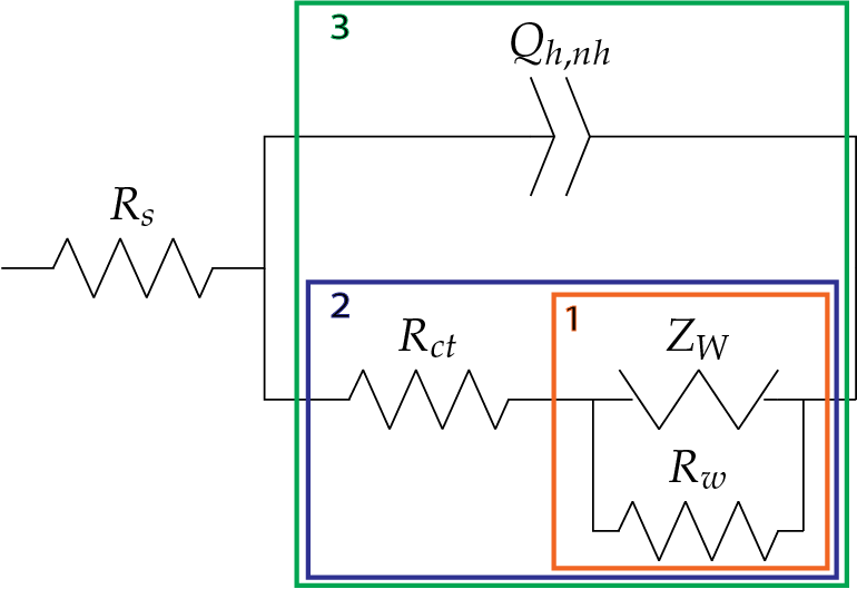
def redox(p, f):
    w = 2*torch.pi*f                # Angular frequency
    s = 1j*w                        # Complex variable
    Rs = p[0]
    Qh = p[1]
    nh = p[2]
    Rct = p[3]
    Wct = p[4]
    Rw = p[5]
    Zw = Wct/torch.sqrt(w) * (1-1j) # Planar infinite length Warburg impedance
    Ydl = (s**nh)*Qh                # admittance of a CPE
    Z1 = (1/Zw + 1/Rw)**-1
    Z2 = (Rct+Z1)
    Y2 = Z2**-1
    Y3 = (Ydl + Y2)
    Z3 = 1/Y3
    Z = Rs + Z3
    Y = 1/Z
    return torch.cat((Y.real, Y.imag), dim = 0)

An even simpler way would be to predefine a function par which computes the total impedance of circuit elements in parallel

def par(a, b):
  """
  Defines the total impedance of two circuit elements in parallel
  """
  return 1/(1/a + 1/b)

def redox(p, f):
    w = 2*torch.pi*f                      # Angular frequency
    s = 1j*w                              # Complex variable
    Rs = p[0]
    Qh = p[1]
    nh = p[2]
    Rct = p[3]
    Wct = p[4]
    Rw = p[5]
    Zw = Wct/torch.sqrt(w) * (1-1j)       # Planar infinite length Warburg impedance
    Zdl = 1/(s**nh*Qh)                    # admittance of a CPE
    Z = Rs + par(Zdl, Rct + par(Zw, Rw))
    Y = 1/Z
    return torch.cat((Y.real, Y.imag), dim = 0)

Tip

The key idea to remember is that for circuit elements in series, we add their impedances while for elements in parallel, we add their admittances.

Next, we define an initial guess, bounds and smoothing factor for each of the parameters as a tensor.

p0 = torch.tensor([1.6295e+02, 3.0678e-08, 9.3104e-01, 1.1865e+04, 4.7125e+05, 1.3296e+06])

bounds = [[1e-15,1e15], [1e-8, 1e2], [1e-1,1e0], [1e-15,1e15], [1e-15,1e15], [1e-15,1e15]]

smf = torch.tensor([100000.0, 100000.0, 100000.0, 100000.0, 100000.0, 100000.0])

Note

The smoothing factor is a value that determines how smoothly a certain parameter varies as A function of the sequence index. The values of the smoothing factor smf are not fixed. They could vary depending on the data and weighting used. Check out the Examples page for more details.

Step 4: Create an instance of the fitting class

An instance our our multieis class is created by passing it our initial guesses p0, frequency F, admittance Z, the bounds, bounds for each parameter, the smoothing factor (smf), the model redox, the weight Yerr and the immittance we are modeling which in this case is the admittance.

eis_redox = pym.Multieis(p0, F, Y, bounds, smf, redox, weight= Yerr, immittance='admittance')

Note

The details of the computation of the standard deviation of the admittance used in this guide is given in this paper. Other methods for obtaining the standard deviation of impedance measurements are briefly described under the Frequently asked questions section. To fit using a different weighting scheme, all we need to is replace the weight argument Yerr with the strings “modulus”, “proportional” or None (i.e unit).

Step 5: Fit the model to data

Once our class in instantiated, we fit the data by calling any of the fit methods. pymultipleis offers a fit_simultaneous(), fit_simultaneous_zero() and a fit_stochastic() method. The fit_simultaneous() and fit_simultaneous_zero() methods have accept two extra arguments: method which can be any of the methods (TNC, BFGS and L-BFGS-B) and n_iter, an integer which determines the number of iterations used in the minimization. fit_stochastic() takes in two arguments, a learning rate (lr) and num_epochs, which for most problems, setting learning_rate = 1e-3 and num_epochs = 5e5 is probably sufficient.

popt, perr, chisqr, chitot, AIC = eis_redox.fit_simultaneous()

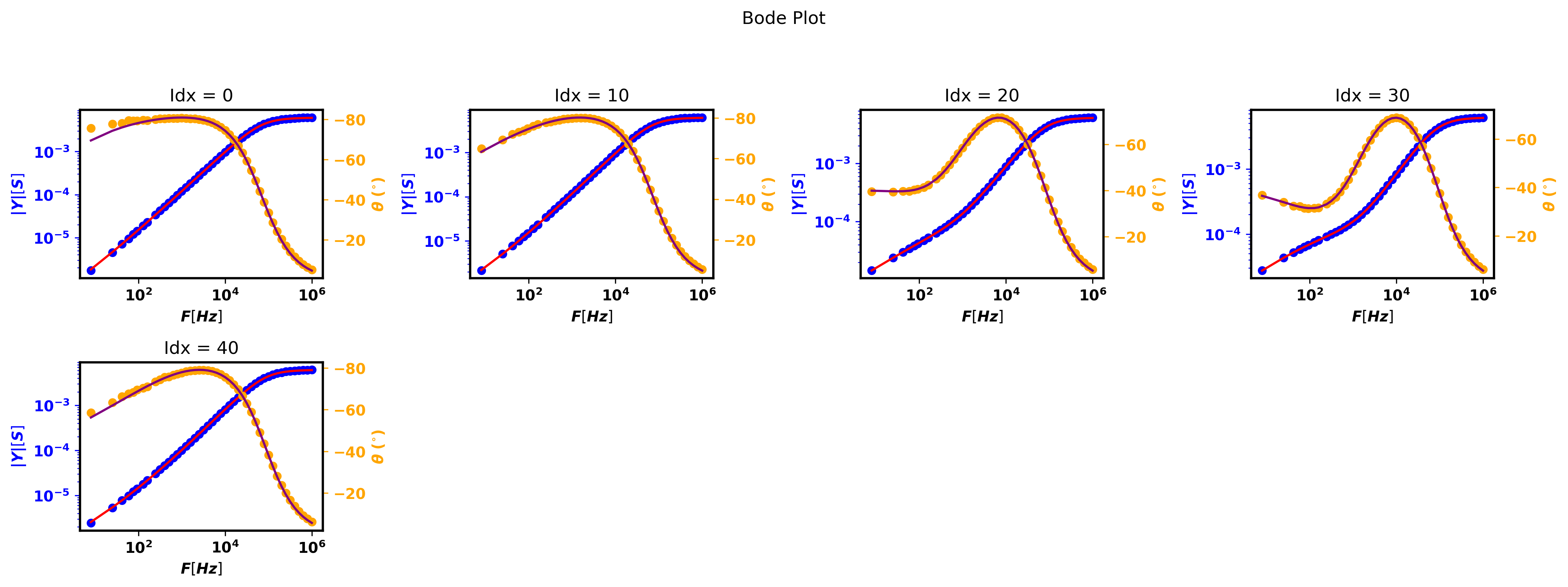
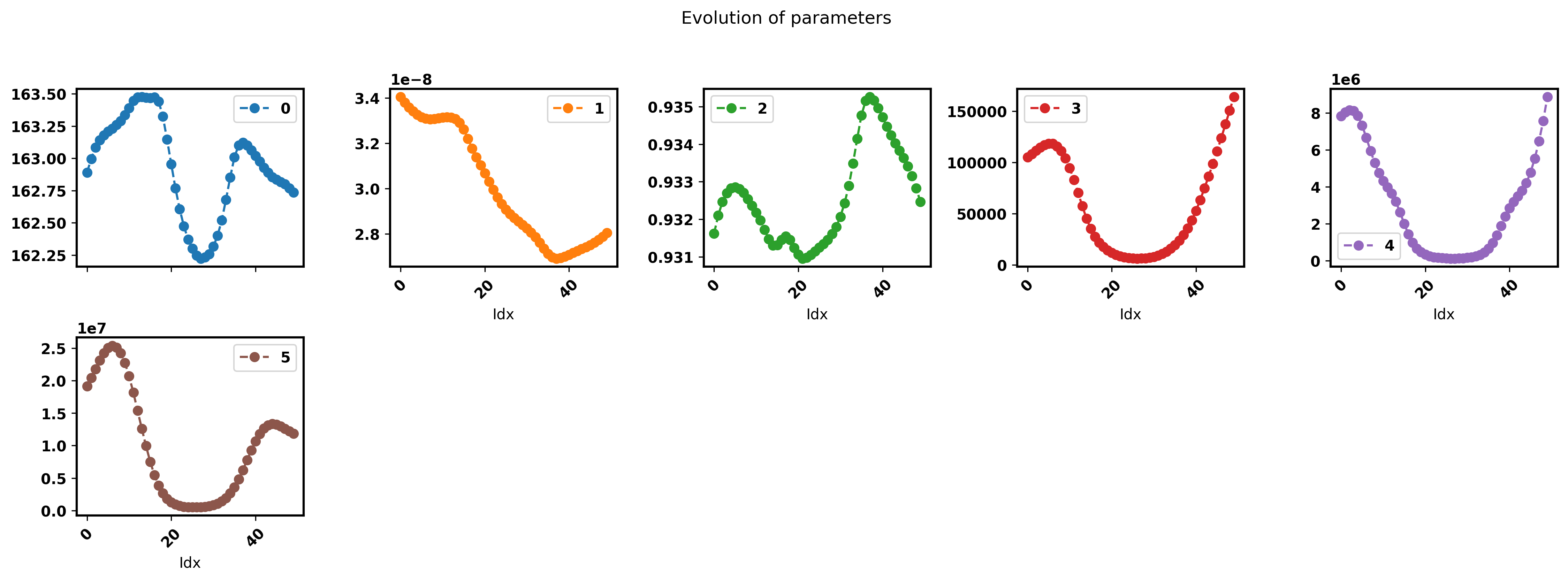
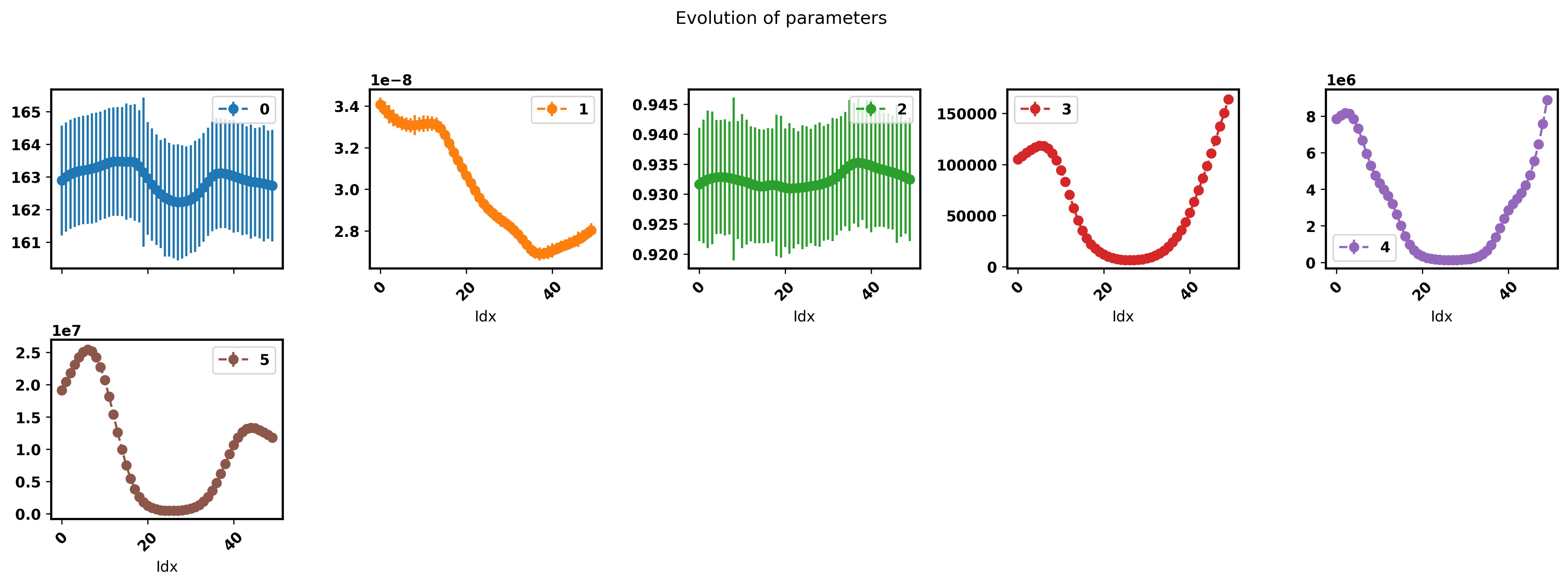
Step 6: Visualize the plots

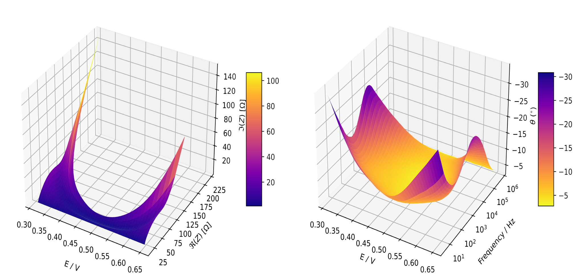
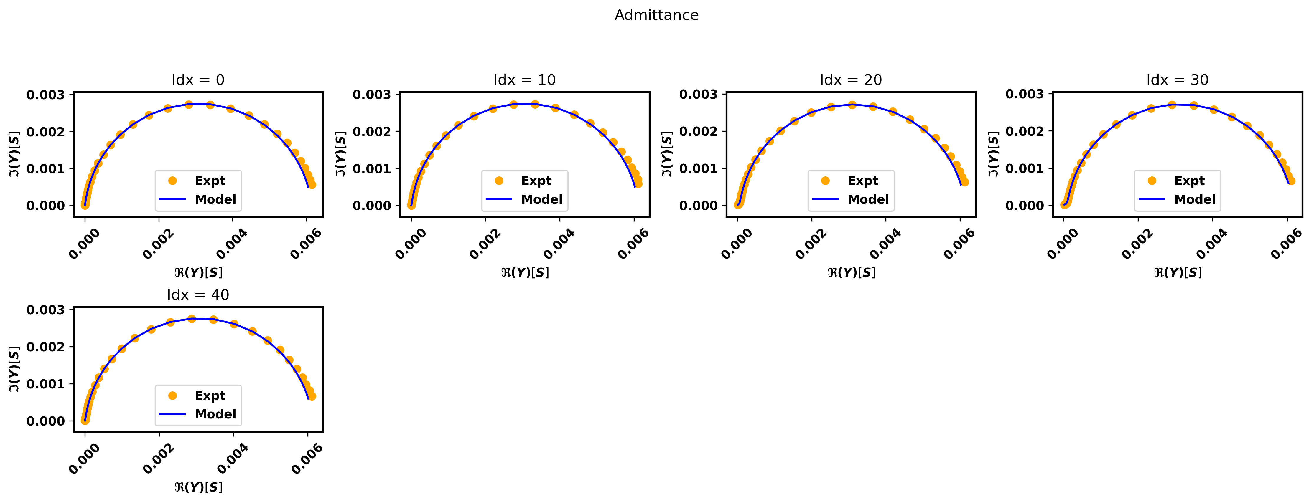
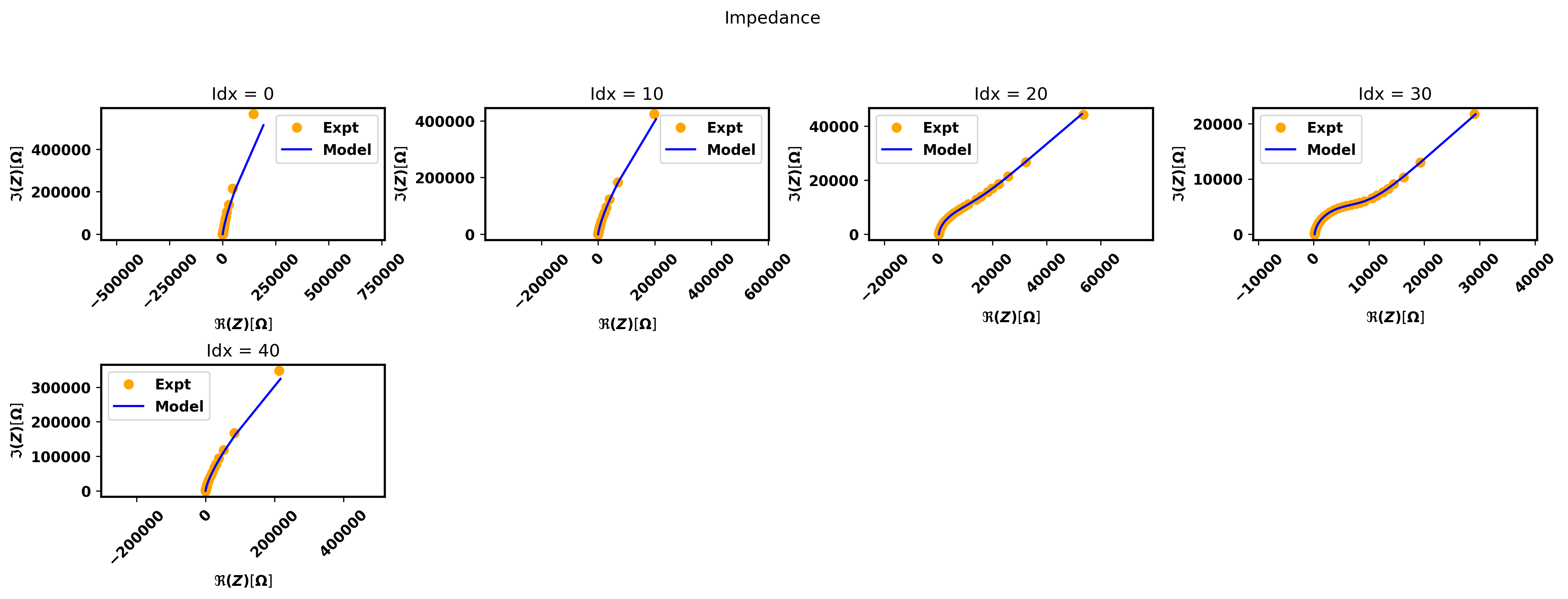
In order to make it easy to visualize the plots resulting from the fitting procedure, pymultieis offers three different plotting methods. We call the plot_nyquist() method on the instance we created to view the complex plane plots, the plot_bode() to view the bode plots and the plot_params() method to view the parameter plot. Thus we have a total of four generated plots:

The complex plane plots (Nyquist) - the impedance and the admittance plots are generated. This method can be called before or after a fit.
The Bode plots - can be called before and after a fit.
The plot of the optimal parameters - can only be called after a fit.

The plot_nyquist() and plot_bode() methods take in a steps argument which determines the interval over which the plots are sampled. The default argument for the steps parameter is 1. A maximum of 20 plots can be shown to avoid cluttering the screen. The plot_params() method has a show_errorbar parameter which accepts a boolean. When set to True, the parameters are plotted with their respective standard deviations shown as errorbars. There is also a labels parameters which accepts a dictionary as argument. The keys represent the circuit elements while the values are the respective units.

eis_redox.plot_nyquist(steps = 10)

eis_redox.plot_bode(steps = 10)

eis_redox.plot_params()

eis_redox.plot_params(show_errorbar=True)

Step 7: Save the results

In addition, pymultieis provides methods to save the generated plots. The save_plot_nyquist() saves the complex plane (Nyquist) plots, the save_plot_bode() saves the Bode plots while the save_plot_params() saves the plot of the optimal parameters. The save_plot_params() can only be called after a fit is performed.

eis_redox.save_plot_nyquist(fname='redox')
eis_redox.save_plot_bode(fname='redox')
eis_redox.save_plot_params(fname='redox')

The is also a save_results() method which saves the optimal paramaters popt, the standard error of the parameters perr, the predicted spectra Z_pred and the metrics associated with the fit i.e. the chisquare and the Akaike Information Criterion AIC. The save methods have an fname parameter which accepts as argument a string representing the name given to the sub-folder within the current working directory into which plots and results are saved. If no fname is provided, a default name ‘fit’ is used. See an example of saving with an fname below.

eis_redox.save_results(fname='redox')

Warning

If a value to fname is specified by the user, it must be used as a keyword argument and must also be a valid string